
Bettors will often focus on the idea of success in betting. People want to fail as little as possible and win as much as they can. Andrew Mack, author of Statistical Sports Models in Excel, believes that failure could be the secret to success in betting. In his debut article for Pinnacle, he explains why.

Failure: The secret to success?
“Nothing in this world can take the place of persistence. Talent will not: nothing is more common than those who are unsuccessful yet talented. Genius will not; unrewarded genius is almost a proverb. Education will not: the world is full of educated derelicts. Persistence and determination alone are omnipotent.” – Calvin Coolidge
When it comes to sports modelling, failure can be the secret to eventual success.
In this article I’d like to walk you through a simple method for deriving the 1X2 outcome probabilities of an NHL game through simulation. To start, we’ll work our way through a basic model template you can run for yourself easily in Excel. The model will be simplistic but functional.
However, my true purpose in sharing this with you is to introduce some of the lesser discussed elements of sports modelling: failure, critical analysis using domain knowledge and troubleshooting.
It can be a surprising truth in model building that you often learn more from your failures than your successes. To that end, once we’ve put this model together and established a basic process, we will critically analyse the model’s weaknesses to look for opportunities to improve it. In doing so I hope to give you something even more valuable in the long term than any one model – a troubleshooting process for improving your own ideas until they are sharp enough to compete successfully. Let’s begin.
Step 1: Gather some data
To start, we’re going to need some data. Let’s head over to Hockey-Reference.com and copy and paste all the game result data from this year’s 2019-2020 NHL season into an Excel spreadsheet.
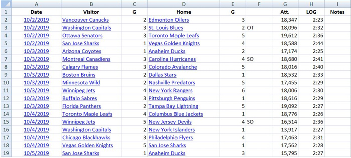 We can accomplish a surprising amount of analysis using only this simple game result data. For example, we might want to know the mean number of goals scored for both home and away teams, the variance of goals scored, or the frequency of overtime.
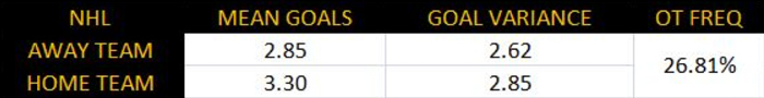
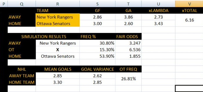
If we use the AVG and VAR functions in Excel, we can see that home teams average 3.30 goals per game while away teams average 2.85 goals. The variance of these goals respectively is 2.85 and 2.62. Overtime so far this season has occurred approximately 26.81% of the time. At the very least, we’ve got our data. Now let’s identify the distribution of our target outcome.
Step 2: Observe the distribution of our target result
Let’s suppose our target outcome is the number of goals scored for each team, which seems fairly straightforward if we’d like to predict who is likely to win and approximately how often. It would be handy to know what sort of statistical distribution this data roughly fits into when we later attempt to turn our forecasted expectations into probabilities.
We know that goals in the NHL are a form of discrete count data. They are relatively rare despite there being many opportunities for success, scored one at a time and containing an element of randomness. The Poisson distribution seems like it would be a natural choice. We can check this with any number of Excel add-ons:
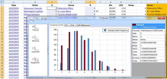
The Poisson distribution appears to be a decent fit for our data. No surprise here, as this has been studied and commented on for years by various statistics researchers. Let’s keep this distribution information in the back of our minds as we move on. It will become useful very shortly.
Step 3: Establish an opponent adjusted expectation for each team
We have our data, we have a target outcome, and we have a probability distribution. Now we need a model structure to get our base forecast for each game. For this example I’ll use a simple model structure that takes the average goals scored for and against each team in the home or away situation and averages them together. The function will look like this:
xGoals For = (Avg Goals For + Avg Goals Against Opponent)/2
Doing it this way, we have accounted for offence, defence, and home ice advantage (albeit in a simplistic way). Using the New York Rangers vs. Ottawa Senators game from November 22, we can see that our model expected Ottawa to score 3.43 goals and New York to score 2.73. Just eyeballing this tells us that our model, given what it knows, expected Ottawa to win.

Step 4: Simulate results to reflect randomness
Now that we have goal expectations for both teams, we need a way to convert these expectations into probabilities. A common way to do this is with a competing Poisson matrix, as I laid out in my book “Statistical Sports Models in Excel”. This is fairly easy to do in Excel using the POISSON function.
One potential downside to this method though is that it doesn’t take the randomness of goal scoring into account very well. In order to try and get a better picture of how this game is likely to end up, we’re going to try something a bit different here by using a Poisson simulation instead. To do this we’ll be using Excel’s random number generation function.
Assuming you have the data analysis toolpack installed in your version of Excel, click on “Data”, then click “Data Analysis” and finally click “Random Number Generation”.
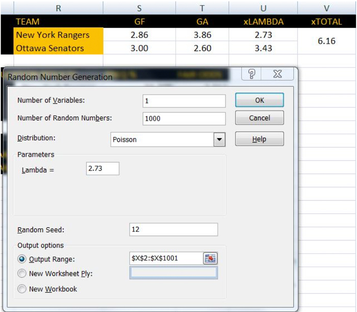
What this is going to do for us is simulate 1,000 games using our goal expectations for each team. We can then calculate the frequency that each team wins, the frequency of overtime, or anything else we might like to know.
Let’s input “1” as the number of variables, “1000” as the number of random numbers (simulated games), “Poisson” as the distribution, and New York’s expected goals (2.73) as the lambda. Once we select the appropriate place on our spreadsheet where we want the results outputted, we click “OK” and let the random number generator work its magic.
Once the simulation is complete, we simply do the same for Ottawa, making sure to output the results in the appropriate adjacent column on the sheet.
Step 5: Convert into probabilities
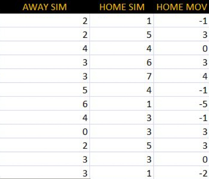
Now that our simulations for both teams are complete, we need to count the frequency of occurrence for a home win, an away win, and a regulation tie. To do this we’ll add an additional column to our sheet which calculates the home team’s margin of victory [MOV]. Then we’ll count how many times out of 1000 the home MOV is greater than zero, less than zero, and exactly zero.
This should give us probabilities we can use to estimate prices for a home win, away win, and a regulation tie. Having done this, the model estimates New York’s fair regulation price as 3.247, Ottawa’s fair price as 1.855, and the fair price on a regulation tie as 6.536. We can then compare these estimated prices to market prices in our search for betting value.
Analysing model weaknesses
Ottawa ended up winning this game in rather emphatic fashion in regulation, but let’s not be too quick to assume that we’ve got a winning model on our hands. Despite a one-off success this model isn’t particularly great. I don’t recommend you bet with this. If we were to use this against the market on a large number of trials we’d be bringing a pair of safety scissors to a gun fight. That much is quite clear to me, and will be clear to you as well if you decide to run a backtest on what we’ve built so far.
What might not be so clear, particularly if you’re a neophyte modeller, is why. This can be a frustrating moment for a model builder. You’ve done some work, created what you think is a reasonably decent process and the result is failure. It may appear as though you’ve invested considerable time and energy trying to make progress only to end up back at the starting line.
But this is not where your model ends. Rather, it is where the real work begins.
A good model is analogous to a good pair of binoculars – it sees far ahead and the resolution is sharp. Poor models don’t see very far ahead (or worse, are looking backwards!) and produce a fuzzy image resolution. Poor performance in a backtest is an indicator that our model is giving us a fuzzy picture of future performance. When that happens, it’s usually a good idea to ask ourselves:
- What variation in the underlying process are we not adequately addressing?
- What assumptions might we be making that are proving disastrous?
- How can we make the picture sharper?
What follows are some suggestions to guide your troubleshooting process. By continuing to improve your model through learning from its failures, you can eventually succeed in making it sharp enough that it becomes a valuable tool in your betting arsenal.
Consider the data
It’s time to strip this model down to the bolts and see what might be wrong with it. Let’s start by considering the data we’ve used. It seemed simple enough – we wanted to project goal scoring, so we used goals. That should work right?
Maybe, maybe not. Goal scoring data is result data. Results in any sport contain an element of noise, which simply means that some proportion of the recorded result is not driven by an underlying repeatable skill that we can forecast accurately.
The more random the scoring in a sport, the proportionally larger this statistical noise is likely to be. In hockey, there is quite a bit. We may have inadvertently attempted to model noise here – which is certainly one reason why our model could be producing poor results.
Think about what you’ve seen in hockey games: Empty net goals, bad bounces that end up in the back of the net, deflections from the point that tip in off a player’s elbow – these are all recorded as goals for a team. Should they be counted as part of that team’s latent ability relative to another team? Probably not. This is where statistical techniques like regression become important, and why an expected goals forecast (xG) is usually considered a more powerful predictor of future success than actual goals.
When you strip away as much noise as possible you can better map the underlying repeatable skills that are causative of goals. Assigning goals that have already occurred to a team’s latent ability in any scenario where there is significant noise is a mistake. Taking that into consideration opens up new possible areas to explore in trying to improve our model.
Takeaway #1: Find ways to reduce noise in your data relative to your target outcome.
Consider model assumptions
Every model you make contains assumptions. When a model fails, it’s quite useful to identify and question those assumptions to see if you can find opportunities to improve them. The first assumption we made in our example was that actual goals are representative of team strength and latent ability. We have reason to believe that might not be the best approach, and we’ve written it down as an area to explore.
What other assumptions have we inadvertently made that might be wise to question?
Let’s consider the Poisson distribution. It seemed like a decent fit for our data, but when we did our initial analysis of goal scoring averages and their variance we observed something interesting: for both the home and away teams the averages and the variances weren’t the same.
In both cases, there appeared to be some under-dispersion occurring. This could be a potential problem, because one of the fundamental assumptions that must hold for the Poisson distribution to be appropriate is that the mean and the variance of the data are supposed to be the same.
If the variance exceeds the mean, distributions like the Negative Binomial are usually a good place to look. If the variance is less than the mean, we might consider the Conway-Maxwell Poisson adaptation.
Additionally, we might find with a larger sample size of games that NHL goal scoring means and variances converge towards being equal. The point is another distribution may be more suitable to what we’re trying to accomplish here. It’s important to be mentally flexible and not just accept a solution without considering other possibilities.
Takeaway #2: Challenge your model’s assumptions in data, distributions and functions.
Consider unaccounted sources of variation
Finally, we might wish to consider sources of variation in the results that we haven’t accounted for. How about some examples? For starters, we’ve assumed that a team’s strength is an undifferentiated mass. That is to say, we aren’t taking key injuries or player substitutions into account. Are the Edmonton Oilers capable of performing at the same level whether Connor McDavid plays or not? Surely there is a significant change in either scenario that our current model is blind to.
Also, we’ve assumed that a team’s goals-against expectation is the same regardless of which goalie is starting the game. That’s not an overly helpful assumption either, as starting goalies and backup goalies have distinct save percentage ranges that are usually different from one another. Both of these considerations represent possible unaccounted for sources of variation that could assist our model in producing a sharper picture.
We might also consider strength of schedule, fatigue, referees, altitude, and a number of other factors our model doesn’t currently take into account. The best sources for clues on where to look come from some degree of domain knowledge. Our model doesn’t know that one team is coming in off a back-to-back with their backup goalie starting and 2 key injuries – but you do.
Takeaway #3: Use domain knowledge to look for sources of unaccounted for variation.
Using common sense and some domain knowledge, we’ve begun to consider how this model might be improved by brainstorming potential reasons why it might fall short in predictive prowess. We can revisit our data, our distribution and our assumptions to find areas full of opportunity for our model to improve. Slowly building on this process and being undeterred by initial setbacks is the path to profitability.
In that way, model failures can blaze a path to your eventual success, provided you learn from your mistakes and don’t give up.
![]()
MORE: TOP 100 Online Bookmakers >>>
MORE: TOP 20 Cryptocurrency Sportsbooks >>>
MORE: Best E-Sports Betting Sites >>>
Source: pinnacle.com